|
RESULTS
The table below resumes the results obtained in our analysis of Mus spretus selenoproteome. All selenoproteins predicted in Mus spretus can be found in this table, as well as the proteins involved in their synthesis. Every protein has been located in a given contig of Mus spretus genome and the exact location within this contig has been identified (columns 1 and 2, respectively).
The relevant documents for protein prediction can be found in the table. These include the results of tBLASTn, T-Coffees obtained with Exonerate or Genewise, SECIS information and the photograph of the chosen SECIS, and Seblastian. Moreover, in the last column we have included the Matlab figures where all blast hits can be seen, together with Exonerate and Genewise predictions (see below for more information). Genewise and Exonerate T-Coffees have only been added when they were accurate and relevant for obtaining the final prediction. In the third column, final protein predictions can be found.
Since we have used both Mus musculus and human selenoproteomes to make our predictions, we have attached the documents obtained from Mus musculus with a mouse icon and the ones obtained from humans with a person icon.

SELENOPROTEINS AND CYSTEINE HOMOLOGUES
|
| Protein Name |
Contig |
Gene Location |
Predicted Protein |
tBlastn |
Exonerate |
Genewise |
Secis Info |
Secis Photo |
Seblastian |
Matlab Figure |
| Glutathione peroxidase (GPx) |
| GPx1 |
CM004102.1 |
109207309-109208129 |
 |
|
|
|
|
|
|
|
| GPx2-a |
CM004106.1 |
70218431-70221164 |
|
|
|
 |
|
|
|
|
| GPx2-b |
CM004100.1 |
89512429-89512994 |
|
|
|
|
|
|
|
|
| GPx3 |
CM004105.1 |
53888501-53895197 |
 |
|  |
|
|
|
|
|
| GPx4 |
CM004103.1 |
78895105-78898745 |
|
|
|
|
| |
|
|
| GPx5 |
CM004107.1 |
17270357-17275565 |
|
|
|
|
|
|
|
|
| GPx6 |
CM004107.1 |
17297628-17304819 |
|
|
|
|
|
|
|
|
| GPx7 |
CM004097.1 |
105404803-105410611 |
|
|
|
|
|
|
|
|
| GPx8 |
CM004107.1 |
110154109-11057254 |
|
|
|
|
|
|
|
|
Iodothyronine deiodinase (DIO) |
| DIO1 |
CM004097.1 |
104286841-104301651 |
|
|
|
|
|
|
|
|
| DIO2 |
CM004106.1 |
84555859-84564721 |
| |
|
|
|
|
|
|
| DIO3 |
CM004106.1 |
105018284-105019117 |
|
|
|
|
|
|
|
|
Thioredoxin reductase (TXNRD) |
| TXNRD1 |
CM004103.1 |
81689812-81714116 |
|
|
|
|
|
|
|
|
| TXNRD2 |
CM004110.1 |
15356078-15410943 |
|
|
|
|
|
|
|
|
| TXNRD3 |
CM004099.1 |
88803548-88833559 |
|
|
|
|
|
|
|
|
Methionine sulfoxide reductase A (MsrA) |
| MsrA |
CM004108.1 |
54488572-54815934 |
|
|
|
|
|
|
|
|
Methionine-R-sufoxide reductase (MSRB) |
| MSRB1 |
CM004111.1 |
21502796-21509320 |
|
|
|
|
|
|
|
|
| MSRB3 |
CM004103.1 |
121537637-121663987 |
|
|
|
|
|
|
|
|
15kDa selenoprotein (Sel15) |
| Sel15 |
CM004096.1 |
144217792-144243497 |
|
|
|
|
|
|
|
|
Selenoprotein H (SELENOH) |
| SELENOH |
CM004095.1 |
84546376-84546943 |
|
|
|
|
|
|
|
|
Selenoprotein I (SELENOI) |
| SELENOI |
CM004098.1 |
27268100-27306511 |
|
|
|
|
|
|
|
|
Selenoprotein K (SELENOK) |
| SELENOK-a |
CM004108.1 |
22613900-22618809 |
|
|
|
|
|
|
|
|
| SELENOK-b |
CM004097.1 |
132604011-132604226 |
|
|
|
|
|
|
|
|
| SELENOK-c |
CM004095.1 |
169487792-169487989 |
|
|
|
|
|
|
|
|
| SELENOK-d |
LVXV01025633.1_8 |
9521-9799 |
|
|
|
|
|
|
|
|
Selenoprotein M (SELENOM) |
| SELENOM |
CM004105.1 |
417415-419622 |
|
|
|
|
|
|
|
|
Selenoprotein N (SELENON) |
| SELENON |
CM004097.1 |
131159360-131172024 |
|
|
|
|
|
|
|
|
Selenoprotein O (SELENOO) |
| SELENOO |
CM004109.1 |
89147087-89157897 |
|
|
|
|
|
|
|
|
Selenoprotein P (SELENOP) |
| SELENOP |
CM004109.1 |
192628-197787 |
|
|
|
|
|
|
|
|
Selenoprotein S (SELENOS) |
| SELENOS |
CM004100.1 |
53733901-53743134 |
|
|
|
|
|
|
|
|
Selenoprotein T (SELENOT) |
| SELENOT |
CM004096.1 |
56410358-56427006 |
|
|
|
|
|
|
|
|
Selenoprotein U (SELENOU) |
| SELENOU1 |
CM004108.1 |
34057328-34066959 |
|
|
|
|
|
|
|
|
| SELENOU2 |
CM004107.1 |
61511789-615300095 |
|
|
|
|
|
|
|
|
| SELENOU3 |
CM004097.1 |
151529697-151532124 |
|
|
|
|
|
|
|
|
Selenoprotein W (SELENOW) |
| SELENOW-1 |
CM004100.1 |
8372322-8374762 |
|
|
|
|
|
|
|
|
| SELENOW-2 |
CM004105.1 |
99815374-99815374 |
|
| |
|
|
|
|
|
MACHINERY PROTEINS
|
| Protein Name |
Contig |
Gene Location |
Predicted Protein |
tBlastn |
Exonerate |
Genewise |
Secis Info |
Secis Photo |
Seblastian |
Matlab Figure |
tRNA Sec 1 associated protein 1 (SECp43) |
| SECp43 |
CM004097.1 |
128762881-128781272 |
|
|
|
|
| | |
|
Selenophosphate synthetase (SEPHS) |
| SEPHS2 |
CM004100.1 |
117216271-1172117623 |
|
|
|
|
|
|
|
|
Selenocysteine synthase (SecS) |
| SECS |
CM004098.1 |
50454061-50480812 |
|
|
|
|
|
|
|
|
Phosphoseryl-tRNA kinase (PSTK) |
| PSTK |
CM004100.1 |
121562581-121571150 |
|
|
|
|
|
|
|
|
SECIS binding protein 2 (SBP2) |
| SBP2 |
CM004107.1 |
48925499-48962157 |
|
|
|
|
|
|
|
|
Eukaryotic elongation factor (eEFsec) |
| eEFsec |
CM004099.1 |
87343010-87537215 |
|
|
|
|
|
|
|
|
We attach a text file with the predicted exon locations and SECIS coordinates for each protein within the contig. We also add a visual representation of this data, which is a Matlab figure that allows the user to browse across through the Mus spretus selenoproteome.
Example of protein prediction
To illustrate the process of prediction we want to show an example. We chose SELENOI because it could be predicted from the mouse query and the analysis is easy to understand.
After data acquisition we generated a Matlab figure that contains the relevant information for screening a candidate protein (every figure is attached in the Results table). Below there is a screenshot of how this figure looks (in this case it refers to the mouse query SPP00001577_2.0):
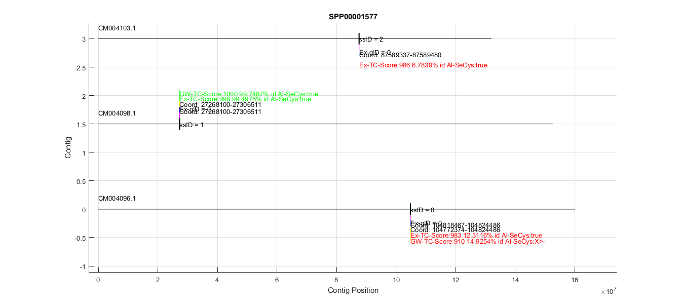
This figure shows the following elements that we got in data acquisition (see methods for a proper understanding of how these files were generated):
- Mus spretus contigs in which we got tBLASTn hits (black lines).
- The location of these BLAST hits (purple boxes).
- The SUBSEQ regions generated from these hits (black boxes).
- Genes predicted by Exonerate (blue boxes, with exons and introns).
- Genes predicted by Genewise (yellow boxes, with exons and introns).
- T-Coffee results for both Exonerate and Genewise predictions(each amino acid is a box with a different color, see below for more information).
Both genes predicted have the locations within the contig annotated. All BLAST, predicted genes and T-Coffee boxes are above or below the contig depending on if they are in the forward or reverse strand, respectively.
The most important thing of this overview figure is the coloring of the T-Coffee text. Each color indicates the homology of the predicted protein to the query (in this case the mouse SPP00001577_2.0 protein). The color code is:
- Red: Less than 30% homology.
- Magenta: Between 30 - 60 % homology.
- Blue: Between 60 - 90 % homology.
- Green: More than 90 % homology.
This allowed us to automatically screen for relevant predictions. In this case there is a very good prediction in contig CM004098.1, and 2 predictions with very low homology. The next step was to zoom into the interesting region to get more information about that prediction. Below is the zoomed CM004098.1 region:
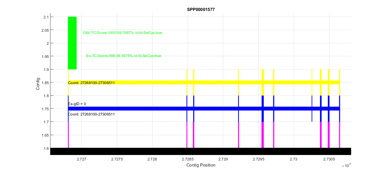
We can see how the BLAST hits, Genewise and Exonerate predictions (first 3 boxes) which overlap completely. The two green boxes are the visual representations of tCoffee mentioned before. The first box (Ex-Tc) refers to the Exonerate T-Coffee, and the second (GW-Tc) refers to the Genewise one. Note that there is a text line that indicates which is the T-Coffee score, the % of homology and information about the alignment of the Sec (in this case it was perfectly aligned, and this is labeled as ''true'').
To understand better how this T-Coffee visual representation works we present the predicted genes in contig CM004096.1, which have very low homology. Below is a zoomed region of the T-Coffee obtained:
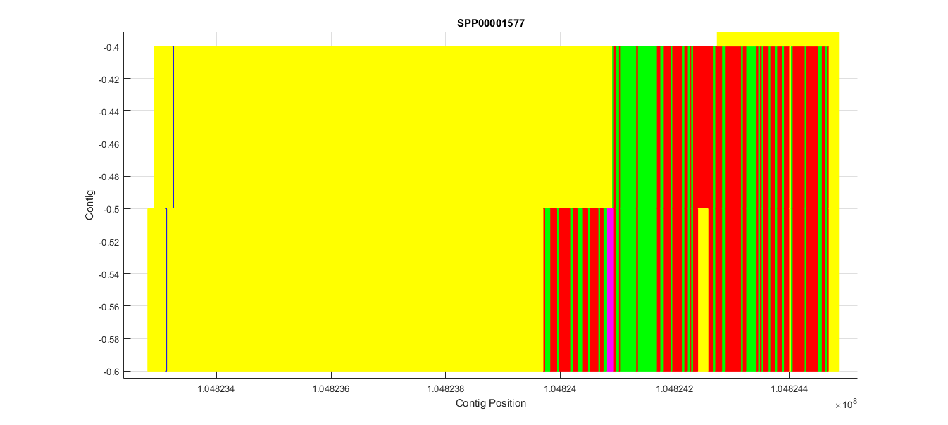
Each of the colors describes how is each query amino acid aligned with the predicted protein:
- Green is match
- Red is miss-match
- Yellow is a gap in the predicted protein
- Purple is a gap in the query protein
There is also a blue outlined box which corresponds to the query Sec. In this case we can see how this prediction had very low homology and the Sec was aligned with a gap (yellow box), so that we discarded it from the analysis.
We used this analysis framework combined with manual verifications to browse among all our files and make precise protein predictions (see discussion for a detailed explanation), in a high-throughput and friendly-interface manner. All figures are attached to the results table.

| |