SelenoDB: Database that contains, among others, the amino acid and nucleotide sequence of selenoproteins that have been predicted in different species. In our case, it is used to extract our query protein sequences, from Danio rerio and Homo sapiens.
tblastn -evalue 0.001 -query -db -out -outfmt "6 qstart qend sseqid sstart send sstrand evalue
tblastn: Allows comparing a protein sequence to a nucleotide sequence, and gives you the e-value of each hit. e-value is a parameter that indicates the expected, how many alignments with this score or higher you could randomly find in a database with the same size and composition. As such, we are looking for a very low value, as it would mean that it is very unlikely for this alignment to take place randomly. In our case, it is used to compare the query proteins (-query) with the genome database (-db) with an evalue lower than 0.001 (-evalue 0.001), and saves the result in a .blast file (-out) that will have a table #6 format(-outfmt "6), with columns with different items (qstart qend sseqid sstart send sstrand evalue).
fastafetch genome.fa genome.index scaffold > Fastafetch.fa
Fastafetch: Allows extracting a single fasta sequence from a multifasta file. In our case, it is used to fish out the scaffold of interest (genome.index) from the whole Haplochromis burtoni genome (genome.fa) and save it in a new file (Fastafetch.fa).
fastasubseq Fastafetch.fa start length > genomic.fa
Fastasubseq: Allows extracting a subsequence from a single fasta sequence. This is interesting when the main sequence is too big for further programs to work correctly (which is the case when the scaffold is this main sequence). In our case, it is used to fish out the region, or subsequence, where our predicted protein is found (Fastafetch.fa) starting from the fastasubseq_start (start) and the potential protein fastasubseq_length (length). Its result is saved in a new file (genomic.fa).
exonerate -m p2g --showtargetgff -q -t | egrep -w exon > exonerate.nuc
exonerate: Allows comparing a sequence (or subsequence) of a genome with a protein query and predicts how this amino acidic sequence could be organized in the genome (exon and intron coordinates). In our case, it is used to determine the coordinates of the exons (egrep -w exons) from a protein query (-q) to a genome target (-t), following as such a protein to genome model (-m p2g). It will save the data in a .gff format (--showtargetgff). However, after selecting only the exons, we ask it to save it in a exonerate.nuc format.
genewise -pep -pretty -cdna -gff -trev query genomic.fa > genewisepredprot.aa
genewise: As exonerate, it allows predicting genes and its regions (introns and exons). However, it is more exhaustive than the previous one. In our case, it is used when exonerate has not worked correctly.
- pep: to show the protein translation
- pretty: to show the pretty ASCII alignment
- cdna: to show the predicted cDNA
- gff: to show the gene prediction in GFF format
- trev: by default, genewise scans in the forward strand. This parameter allows to scan in the reverse strand.
fastaseqfromGFF.pl genomic.fa exonerate.nuc > fastaseqfromGFF
fastaseqfromGFF:Allows obtaining, from a GFF format document, the nucleotide sequence from the predicted exonerate file. In our case, it is used to determine the nucleotide sequence of the exons (exonerate.nuc) parting from the genome of the fish (genomic.fa) and saves it in a fastaseqfromGFF format file.
fastatranslate -F 1 fastaseqfromGFF > predprot.fasta
fastatranslate: Allows obtaining an amino acid sequence from a nucleotide sequence. In our case. It is used to translate the nucleotide sequence of the predicted Haplochromis burtoni genes (fastaseqfromGFF) to its corresponding amino acid (protein) sequence, in a predprot.fasta format. -F 1 tells the program to start reading from the first position of the document.
t_coffee query predprot.fasta > tcoffee.fa
t-coffee: Allows to align two sequences, and among others, gives you the score of this alignment (SCORE = 1000 is a perfect allignment). In our case, it is used to align our predicted Haplochromis burtoni protein (predprot.fasta) to its query protein (query) and saves it in a tcoffee.fa format.
Fig 1. Workflow of the procedure to analyze the selenoproteins 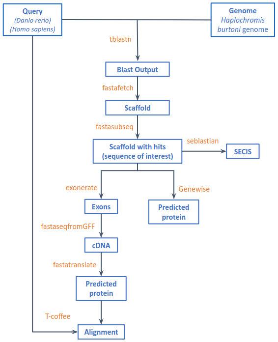
In order to predict, characterize and analyse the selenoproteins found in our species, Haplochromis burtoni, a homology-based study was performed using the SelenoDB public project release 2.0 (the latest available version).
To determine which protein query we should use, we looked for the species that had the most recent common ancestor to ours, and determined that this was Danio rerio, commonly known as zebrafish.
Those proteins that were not optimal in zebrafish (protein does not start with methionine) were taken from Homo sapiens.
In case of a tie (more than one available sequence for each protein), we have supposed that all proteins were paralogues (consequence of a duplication event) so we selected those that both started with methionine and had the longest length (so as to have more possibilities of alignment).
Asides from the 41 selenoprotein-related genes mentioned in the project instructions, we have also decided to look for all the other selenoproteins (or related) present in Danio rerio. As such, this is a list of the proteins that we have screened:
DI, DI1, DI2, DI3, eEFsec, Fep15, GPx, GPx1, GPx2, GPx3, GPx4, GPx5, GPx6, GPx7, GPx8, MsrA, PSTK, SBP2, SECp43, SecS, Sel15, SelH, SelI, SelJ, SelK, SelL, SelM, SelN, SelO, SelP, SelR, SelR1, SelR2, SelR3, SelS, SelT, SelU, SelU1, SelU2, SelU3, SelV, SelW, SelW2, SPS, SPS1, SPS2, TR1, TR2, TR3.
Sequences for each protein were placed in a text file with FASTA format (single-line description started with a > followed by the protein sequence) named query.txt.
Atypical characters (# and %) present in the sequences were also removed in this step.
On a different note, to be able to compare these query proteins to our fish, we needed to access its genome, which was given to us. It can be retrieved through this path:
/mnt/NFS_UPF/soft/genomes/2021/Haplochromis_burtoni/genome.fa
From this point onwards, the analysis of all the proteins was done automatically by running a Python program.
Remark 1: We have used biopython, os and pandas tools and modules to be able to develop our program.
Remark 2: To ensure that all the os module commands were working properly, we also defined a function (run_cmd), which printed an error message ("The command '%s' did not work"%cmd) when the command did not work to ease error tracking. This can be done due to a property of os, which prints automatically a 0 if a command does not work or a number different to 0 when it does.
Remark 3: Before creating any document, we defined a line of code that only executed the mentioned command if the file was not already present (if not os.path.isfile()).
Once the query.txt file was filled with all the query proteins, we parsed each of the FASTA entries (record) using SeqIO and changed the id of each record to the proteinname_queryspecies, and created a folder with this name (which would then contain all the generated files from each query). Once the record’s id was settled, we moved to change any “U” (selenocysteine) from the record sequence to an “X” (tblastn does not recognize selenocysteines). These changes were then applied to a new generated file, queryprotein.fasta.
Up next, we ran tblastn, asking for hits with an e-value lower than 0.001 (mentioned during the seminar sessions) and results in a table format, containing the coordinates of the start and end of the query (protein) and the subject (Haplochromis burtoni genome), the subject id (scaffold), strand (+ or -) and e-value. Once generated, we opened it in a pandas Dataframe, which allowed us to analyse it and edit it.
One query protein could contain more than one predicted protein, so it’s important to separate the tblastn hits in scaffolds and strands. To do so, we made a new Dataframe (df_scaffst) containing a single scaffold and strand, and filtered the coordinates from the subject start column in ascending (+ strand) or descending (- strand) order.
As it happened in the previous iteration, different hits found in the same scaffold and strand could ultimately belong to different proteins. To separate them, we decided to make this fourth loop, which iterated through each row of the df_scaffst query start column and defined the start and end of each single predicted protein (in a list of lists variable). Remark: This loop is done asides from the next iteration, so this is why values are stored in a variable where each position contains a list (start and end for each single predicted protein).
Once the previous loop is completed, the program moves into this fifth loop, which contains the commands to process these single predicted proteins from tblastn. After redefining the genomic start and end coordinates for the fastasubseq, we executed Fastafetch to fish out the sequence of the scaffold of interest, and saved it in a Fastafetch.fa format (preceded with the pertinent protein_name, scaffold, fastasubseq_start, fastasubseq_end data).
Note: All documents generated using the Materials programs will all be preceded by these data. However, to avoid reiterations, we just mention the format change for each file.
Remark: The genomic start and end coordinates obtained from the tblastn were extended (-50.000 bp for the start and +50.000 for the end), because blast's local alignment algorithm rarely retrieves protein queries as a unique hit. Instead, each exon or each highly identical portion between the query and the genome is reported as an individual hit. In consequence, if this extension is not performed, some poorly-conserved exons might be lost.
Next, we ran Fastasubseq, which allowed us to extract the desired region from the whole scaffold sequence, by giving it the fastasubseq_start position (tblastn_start - 50.000 nt) and length (fastasubseq_end - fastasubseq_start). It was saved in a genomic.fa format.
Now that all documents are in the desired format and content, we proceeded with exonerate, and obtain the coordinates of each of the single predicted protein exon start and end, saved in a exonerate.nuc format.
Note: if the alignment is of a very poor quality, exonerate gives no results, and as such, the exonerate.nuc file is empty. As such, we made a conditional statement that, for these empty files, does not execute exonerate, but genewise. However, as its alignment is so poor, its processing stops here; the following last steps are just for those predicted proteins that have executed correctly exonerate.
Once exonerate was complete, we followed by fastatranslate, and once we obtained the amino acid sequence of the Haplochromis burtoni predicted protein and saved it in a predprot.fasta format, we proceeded to execute the last program, tcoffee. It allowed us to compare our predicted protein to our query, and saved the alignment results in a tcoffee.fa format (including the alignment score).
Asides from saving all the generated documents in a folder (named query protein) we also decided to generate an automatized table containing the protein name, scaffold, start and end fastasubseq coordinates and strand from the predicted Haplochromis burtoni selenoprotein-related genes, species of the query used, and whether the Haplochromis burtoni or Danio rerio protein sequence contained selenocysteine (U), cysteine (C). If the protein did not exist in zebrafish, a hyphen (-) is found in this last column. All of this data was saved in a csv file (selenocistein_table.csv).
Once all the predicted proteins were obtained, we analysed the potential candidates of each type of protein (more details in Results) and we then predicted whether the sequences were actual selenoproteins and/or contained SECIS elements, by using SEBLASTIAN or SECISearc3 respectively.
Moreover, we also performed some phylogenetic analysis in the shape of trees using phylogeny.fr. We compared our predicted proteins with our two queries, Danio rerio and Homo sapiens.
The selenoproteins of Danio Rerio were used as a query because both Danio Rerio and Haplochromis burtoni are classified in the Class Actinopteri, being D. Rerio closer to H. burtoni than H.sapiens.
The proteins used as a query are shown in the following table:
| Origin | Selenoproteins |
|---|---|
| Homo sapiens | Sel15, GPx4, GPx7, GPx8, DI1, PSTK, SBP2, SelI, SelM, SelU2, SelU3, TR2 |
| Danio Rerio | Fep15, eEFsec, GPx2, GPx3, GPx, DI, MsrA, SecS, SPS, SPS2, SelH, SelJ, SelK, SelL, SelN, SelO, SelP, SelR1, SelR2, SelR3, SelR, SelS, SelT, SelU, SelW, TR3, SECp43 |