METHODS

The aim of this project was to perform a prediction and annotation of Urocitellus parryii's selenoproteins, selenoprotein machinery factors and proteins related to selenium metabolism. In order to do that, we decided to do a comparison with the human genome, considered to be the most suitable reference genome (see Obtention of the Human’s genome ). To accomplish this, a set of bioinformatic resources have been used, which will be explained throughout this section.

We present in here an scheme describing the steps followed through the development of the project:

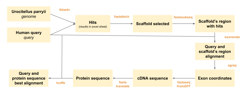
Figure 1. Scheme that describes the protein prediciton process.

Obtention of Urocitellus parryii's genome

The Urocitellus parryii's genome (genome.fa) was offered to us by the lecturers of ‘Bioinformatics’ module, as a Fasta file found in the directory:

/cursos/20428/BI/genomes/2018/Urocitellus_parryii/genome.fa

Obtention of the Human's genome

The next step was to acquire the human's selenoproteins and some other related proteins, which were obtained from the SelenoDB 1.0 website and we recopilated them in a multifasta file named ‘selenoproteineshuma.fa’.

The human genome was used as reference, since we considered it was the one that best suited our requirements: relatively close in the phylogenetic tree, including more selenoproteins and proteins of interest than Mus musculus’ genome (which was also considered at first). Besides, the human genome will always be preferably chosen to any other genome (as long as it makes sense to use it), since it has the best annotation. The U’s (indicating presence of selenoproteins) were then replaced by X’s.

Eventually, every query protein was placed in single fasta files, by using the programme: “ClassifProtsHuma.pl”.

Programming

Several bioinformatic tools have been used to obtain the proteins’ predictions, as indicated in Figure 1. In order to automatically obtain the files needed for the interpretation of the prediction process, two perl scripts were designed:

-Programa_definitiu.pl
-run_all.pl

Actually, ‘Programa_definitiu.pl’ is run within the ‘run_all.pl’ programme, so that we just have to run ‘run_all.pl’ in the shell in order to do the predictions. ‘Programa_definitiu.pl’ codes for the automatization of fastafetch, fastasubseq, exonerate, fastaseqfromGFF, fastatranslate and tcoffee.

‘run_all.pl’ allows to scan the excel sheet were the tblastn results are noted (See BLAST section) and run every selected scaffold along this different programmes.

Data adquisition

An explanation of the different steps will be done in order to have a better understanding of the development of our prediction process. First of all, the loading of the program modules had to be done every day when entering a new computer, as well as giving the suitable permissions before running the Perl script, using the following command within the shell:

Export paths:
- export PATH=/mnt/NFS_UPF/bioinfo/BI/bin:$PATH
- export PATH=/mnt/NFS_UPF/bioinfo/BI/soft/genewise/x86_64/bin:$PATH
- exportWISECONFIGDIR=/mnt/NFS_UPF/bioinfo/BI/soft/genewise/x86_64/wise2.2.0/wisecfg/

Giving permissions:
- chmod u+x * Programa_definitiu.pl
- chmod u+x * run_all.pl

BLAST

BLAST (basic local alignment search tool) is a tool used to compare genome sequences in order to obtain the most significant hits between the sequences we are comparing. A subtype of BLAST, called TBLASTN compares a genome sequence with proteins used as queries. tBLASTn has been run in order to compare each selenoprotein (or orthologous proteins) or proteins involved in selenoproteins machinery of the human database with the genome of Urocitellus parryii. This way, we will obtain the region of our genome of interest which will potentially codify for these proteins in case they exist in Urocitellus parryii. The command used has been:

tblastn -query $prot.fa -db /mnt/NFS_UPF/bioinfo/BI/genomes/2018/Urocitellus_parryii/genome.fa -evalue 0.001 -out $prot.blast -outfmt 7

The output of the programme was a table in which the best hits within different scaffolds were presented. Note that the hits had already gone through a sorting process: hits with e-values less than 0,001 were not selected, which was indicated in the command line of the tblastn. Each column of the table obtained showed different information: name of the protein, name of the scaffold, percentage of identity, length of the alignment, mismatches, gap opens, start of alignment in query, end of alignment in query, starting position of the hit, ending position of the hit, e-value and bit score.

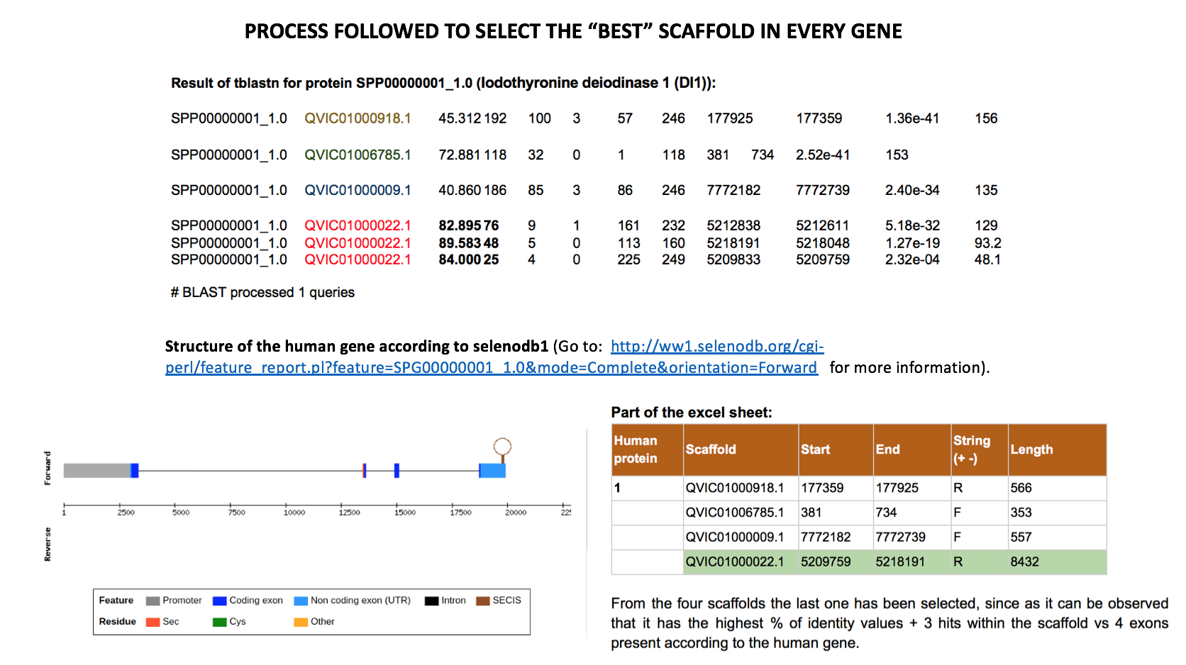
Another aspect to take into account was that for each different scaffold one hit or multiple hits could be found. An excel table was created in order to write down the start and end position of each of the hits and, in case multiple hits were found for one scaffold, a clustering of the hits was manually performed (ie, writing down as start position of the cluster of hits the smallest value of all the starting points within that cluster of hits, and applying the same procedure with the ending points). Doing this manually caused a bit of trouble in the cases where a lot of hits were found within the same scaffold, so in this specific clusters of hits we run a perl programme which selected the maximum and minimum positions (minmax.pl). This way, we finally obtained one starting point and one ending point for each of the scaffolds of all the proteins examined.

Afterwards, a selection of the best cluster of hits for each protein was done (values marked in green in our excel sheet). This selection was performed bearing in mind which cluster had the best % of identity value, which had similar number of hits to number of exons per gene in the human database (number of exons for each gene can be found in: ww1.selenodb.org) and in which the length of each hit slightly suited the length of each exon.

Eventually, we finally selected the best scaffold (cluster of hits) for each protein, so that we will base our final prediction on the one selected here. In some controversial cases more than one scaffold was selected and underwent the following steps of the programme.

However, this methodology has some limitations and we are aware of it, but because of the lack of time we were not able to correct this. The principal limitation would be the inability of finding gene duplications, since we will finally select the prediction based on one scaffold per protein. This method also enables to take a proper prediction if a protein was coded between two scaffolds. Moreover, the selection of the ‘best’ scaffold was not always that easy. Eg, in big family proteins such as GPX, some scaffolds were repeated across the different proteins, being in some cases the same cluster of hits the one we would, at first, select as the best. Having born this in mind, the same scaffold has not been selected for different proteins.

Finally, the scaffolds selected were written down in another Excel sheet, separated by comas and used to automate the procedure for all the proteins.

Here we present an exemplification of the ‘best’ scaffold selection process.

Fastafetch: extraction of scaffold of interest

Now that we know the scaffolds of interest, we need to extract them to a different fasta file, and to do that we will use the program fastafetch (using the database given in the directory mentioned before), with the command:

fastafetch /cursos/20428/BI/genomes/2018/Urocitellus_parryii/genome.fa /cursos/20428/BI/genomes/2018/ Urocitellus_parryii /genome.index $scaff > $scaff.scaffold.fa

The output of the programme was classified in different fasta files, named each one with the name of the specific scaffold as follows: $scaff.scaffold.fa.

Fastasubseq: extraction of exact region of interest

Once we have the scaffolds within different fasta documents, the exact region of the scaffold we want to analyse will be extracted. This region is predicted from the tblastn results.

Note that the extraction of the region was not done taking into account the initial and final positions of the tblastn excel sheet, but extending the search 50.000 nucleotides upstream and downstream these positions, so that we would not miss part of the sequences because of the possible presence of introns (since the hits just represent the coding part of a gene). The addition of these nucleotides was included within ‘Programa_definitiu.pl’.

However, this might lead to errors, since we could overcome the scaffold’s length either in 3’ or 5’. Bearing this in mind, we modeled the programme so that if the final position of our region of interest after adding the nucleotides was larger than the final position of the scaffold itself, the final position of the scaffold itself would be assigned as the final position of the region of interest. The same procedure was applied in the other extreme, assigning a ‘1’ to our initial position in case the result of subtracting 50.000 nucleotides was negative.

The command used for the fastasubseq is:

fastasubseq $scaff.scaffold.fa $pi $llarg > $scaff.subseq.fa

Being $scaff.scaffold.fa the result of the fastafetch (complete scaffold), $pi the initial position selected as explained above and $llarg the length of the region of interest. The output was redirected to fasta files names as $scaff.subseq.fa.

Exonerate and egrep function

Now that we have the subseqs of the scaffolds selected, the programme ‘Exonerate’ will allow us to predict the gene coordinates and the exon coordinates within every single gene predicted. It is important to take into account that, since we first used clustering of hits within every scaffold and not just single hits, more genes will now be predicted (since the region of interest will be larger as well). Moreover, we considered that making the prediction with every gene that resulted from the exonerate output (and not just one) was a better approach, since afterwards a better selection of the prediction that best describes our protein could be done.

A perl script was developed within ‘Programa_definitiu.pl’ in order to automate this. The tough step was to first separate each gene’s information within different fasta documents so that we could afterwards run an ‘egrep’ function to cluster all the exons within every gene.

The command used for the ‘exonerate’ was:

exonerate -m p2g --showtargetgff -q ./proteins_human/$prot/$prot.fa -t $scaff.subseq.fa > EXONERATE.raw

Being ‘EXONERATE.raw’ the output of the exonerate.

The egrep function was also run for every gene as described above:

egrep -w exon $gene_filename > $gID.exon.gff

Being $gene_filename the files were every gene is written down, and $gID.exon.gff the selection of exons in every gene.

Please go to ‘Programa_definitiu.pl’ (exonerate section) for more information and detail of the process followed.

Fasta seq from GFF

This command will be used to extract the cDNA sequence that encodes for the predicted protein and save it into a new document.

fastaseqfromGFF.pl $scaff.subseq.fa $gID.exon.gff > $prot.$scaff.$gID.nucl.fa

Fasta translate

This program will translate the previously obtained cDNA coding sequence into amino acids. The command used:

fastatranslate $prot.$scaff.$gID.nucl.fa -F 1 > $scaff.$gID.pep.fa

Substitution of ‘*’ for X’s

It is relevant to mention that the results obtained from fastatranslate will show the selenocysteine amino acids as "*", which will produce an error when running T-coffee (next step). To fix this, with this command all the "*" are changed in the new file into X's:

sed 's/*/X/g' $scaff.$gID.pep.fa > $scaff.$gID.pepX.fa

T-coffee

T-Coffee has been used in order to perform a global alignment between our final predicted protein from Urocitellus Parryii ($scaff.$gID.pepX.fa) and the query protein from the human’s genome, obtained originally from Seleno DB1 (More information in: ‘Obtention of the Human's genome’). The command used was:

t_coffee $scaff.$gID.pepX.fa ./proteins_human/$prot/$prot.fa > ./proteins_human/$prot/$scaff.$gID.tcoffee.txt 2> ./proteins_human/$prot/t_coffee_$gID.stderr.txt

Two redirections of the output were performed within the command itself, so that two fasta files from the T_Coffe will be directed to the specific folders of each protein: one for the global alignment and another for the errors. This way, in case something goes wrong, a trace-back could be done in order to try to infer what happened. These error files will not be included in our results part since they do not offer relevant information to the alignment itself.

SECISearch3 and SEBLASTIAN

Finally, a secis prediction was also performed. The programmes Seblastian/SECISearch3 were used to do so, using as the input the result of the subseq. Preferably, Seblastian was chosen since its output gave more accurate predictions. Nevertheless, in some cases Seblastian did not find predictions, so SECISearch3 was used (these tools can be found in: http://seblastian.crg.es/).

As it has already been explained, the Secis element is an essential structural motif for the translation of UGA codons into Selenocysteine and not stop codons. This is why it is so important to perform this prediction. The positions of the predictions where noted in an Excel sheet and then compared with the absolute positions of our predicted genes. This is important in order to figure out if the predicted Secis element is found in 3’ position, since otherwise it will be dismissed. In some cases, more than one suitable Secis prediction was found.

Phylogenetic trees

Phylogenetic trees for each protein family were also obtained in order to have the family proteins represented and allowed us to visualize and biologically interpret the results. Moreover, the phylogeny helped us to double-check whether the scaffolds where our gene prediction was done do correlate with the phylogeny or not, judging till which extent our prediction was orthologous to the human protein. The input was the human protein and our protein predictions (the tool used can be found in: http://www.phylogeny.fr/simple_phylogeny.cgi).