In order to find selenoproteins, homologous proteins with cysteine and specific machinery in Anarrhichtys ocellatus proteome, we studied homology of sequences in relation to a model animal. Said model animal was Danio rerio, commonly known as Zebrafish, and it was chosen due to the close phylogenetic relationship with the wolf-eel.
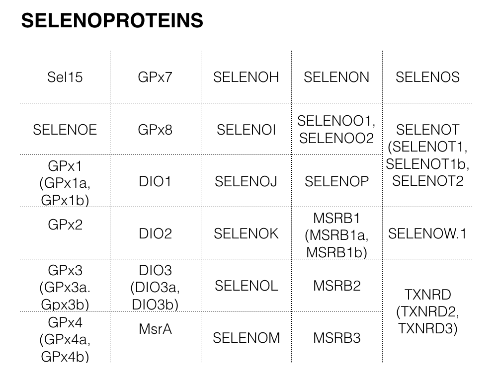
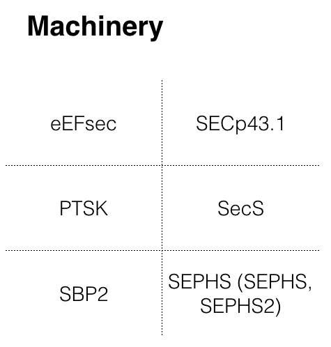
The first step was to search for Zebrafish’s selenoproteins and machinery in SelenoDB 2[9]. The following proteins sequences could be extracted from that database:


Note that, of those proteins with more than one isoform, the longest isoform of the protein was chosen.
Anarrhichthys ocellatus’ genome sequence was already given to us and could be found in this source:
/mnt/NFS_UPF/soft/genomes/2019/Anarrhichtys_ocellatus/genome.fa
The index that worked as a database for our searches was also provided in this other source:
/mnt/NFS_UPF/soft/genomes/2019/Anarrhichtys_ocellatus/genome.index
We then proceeded to make a new Perl program that compared Zebrafish selenoproteome with wolf-eel’s and predicted possible selenoproteins found in our animal of study.
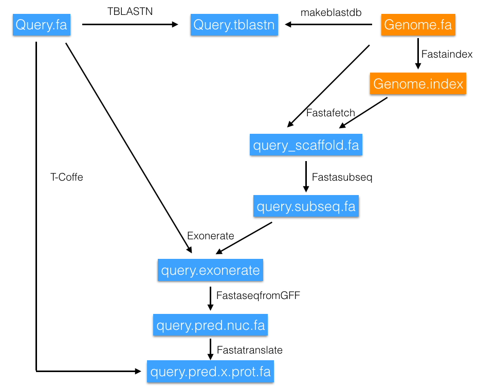
First, our program changed the U residue in Zebrafish’s selenoprotein sequence for an X, and saved that as a file name_protein.fa. That file was our query. This step was necessary because there are softwares that do not recognise U and are not able to work with that residue.
Next, it ran a TBLASTN, a program that compared the protein query to our subject and gave us all the scaffolds found with significant hits. To make our program more efficient, scaffolds with an E-value larger that 0.01 were discarded. The selected scaffolds were redirected to a file name_protein.potential.group.scaffolds.fa.
The next command was FastaFetch, and was used to extract the scaffold of interest from Anarrhichtys ocellatus’ genome. This command needed the information of the subject’s genome, the index and the name of the scaffold. The output was saved in a name_scaffold.fa file.
Once the scaffold was obtained, using Fastasubseq enabled us to extract the region of interest (contig) from the scaffold. The size of our search had to be extended in order to avoid missing part of the sequence due to the presence of introns, so 50,000 more nucleotides were added at both ends of the contig. Some scaffolds were too small for that addition of bases, so in those cases, we used the whole scaffold for the following steps. The output file was saved as name_protein.name_scaffold.subseq.fa.
Next step was running Exonerate, which generated a file with the exons of the protein of interest and stored it in name_protein.name_scaffold.exonerate.gff.
Fasta seq from gff was used to generate a fasta file with the cDNA of the predicted protein from the gff file provided by exonerate. The result was a nucleotide sequence called name_protein.name_scaffold.pred.nuc.fa.
Fasta translate translated the cDNA nucleotide sequence into a protein sequence. The residue encoded by the UGA codon (U) was represented by a *. In order to compare it later with the query sequence (from Zebrafish) it had to be changed to an X. The new file was name_protein.name_scaffold.pred.x.prot.fa.
The last step of the program was T-Coffee, which allowed us to perform a global alignment between the predicted protein sequence and the query protein from Zebrafish. The output was stored in name_protein.name_scaffold.tcoffee.
Our program was automatic, the only variable that the user had to introduce was the name of the protein of interest. The program was able to check all scaffolds with an E-value lower that 0.01 and calculate the length of the contig at the fastasubseq step.
Next, a phylogeny analysis was carried out using phylogeny.fr. The product was one phylogeny tree per protein family and another one per protein in order to see what scaffolds were more closely related to the animal of reference.
The scaffolds to continue our study were chosen based on 1) the quality of the alignment (T-coffee) and 2) the phylogenetic relationship with our animal of reference, the Zebrafish.
A T-coffee with a score higher than 900 and more than 50% coverage was considered good.
The quality of the alignment was a priority to choose the scaffold, there are cases were we used scaffolds with better T-coffees even though they were phylogenetically more distant.
Afterward, the program Seblastian used SECISearch3 to predict SECIS elements in our subject organism and found possible selenoproteins[6]. In order to find SECIS elements in the 3’UTR region of the protein, the input file in that program was the fastasubseq.
When Seblastian could not run because the sequence size was too large, the fastasubseq sequence was cut. Cutting the forward strand was done by selecting the last nucleotide of the scaffold and adding 100,000 more. Conversely, cutting the reverse strand required selecting the first nucleotide and adding 100,000 more.
The output of Seblastian were different files with information about the predicted SECIS elements and some predicted selenoproteins. When multiple SECIS were predicted, the correct ones were found by calculating their positions and making sure they were in the 3’UTR region of the protein.
The last step was the production of the images of the genes structure. The exon drawings were produced based on the exonerate file, which gave information about the location of the gene, the direction and the number of exons it contained. Based on the presence or absence of SECIS elements predicted by Seblastian, those were or were not added to the drawing.
(Note that throughout this process intermediate files were created but were not defined as relevant).