Sequence coding statistics

Bioinformàtica. UPF

Sequence composition bias in coding sequences

Let's perform a very simple exercise: given a nucleotide sequence, compute the number of times that the nucleotide A (Adenine) appears at a distance k from another nucleotide A. And let's do that for every possible k, from 0 to the length of the sequence. For instance if the sequence is

TAAGAGACTCATAAGT

these numbers are

	 K
	 0	 2
	 1	 3
	 2	 2
	 3	 2
	 4 	 1
	 5 	 2
	 6 	 1
	 7 	 2
	 8 	 2
	 9	 1
	10	 2
	11 	 1
	12 	 0
	13 	 0
	14 	 0
	15       0

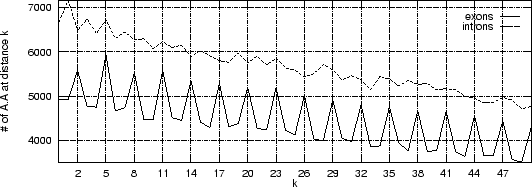
Let's repeat this exercise now for about 500 exon and 500 intron human sequences (actually only 200 bp taken from each exon, and each intron), and let's plot the cumulative frequency of occurrency of pairs A ... A at each possible distance k.

As it is possible to see, a clear periodic pattern arises from the set of exon sequences. The nucleotide A is more likely to be found at distance k=2,5,8, ... from another A than at other distances. This periodic pattern is absent in the intronic sequences.

Note that nucleotide pairs at a distance of k=2,5,8, ... nucleotides, are at the same codon position, whereas nucleotide pairs at other distances, are not.

This periodic pattern reflects the fact that proteins use the different amino acids with different frequencies, and that synonymous codons are used with different frequencies to code for a given amino acid. This causes coding sequences to exhibit an strong codon bias, which is (mostly) absent in non-coding sequnces. The codon bias causes the periodic pattern observed in coding sequences. This periodic pattern is characteristic of the 16 pairs of nucleotides, and not only of the pair A ... A.

Thus, measuring the strength of the periodic pattern in a sequence problem, we can measure the likelihood of the sequence being coding. A measure of DNA sequence periodicity is what we will call here a sequence coding statitic.

coding statistics

A coding statistic or codig measure can be defined as a function that computes given a DNA sequence a real number related to the likelihood that the sequence is coding for a protein.

Since the early eighties, a great number of coding statistics have been published in the literature. Most such coding statistics measure either codon usage bias, base compositional bias between codon positions, or periodicity in base occurrence (or a mixture of all them).

codon usage

Unequal usage of codons in the coding regions appears to be a universal feature of the genomes across the phylogenetic spectra. This bias obeys mainly to (i) the uneven usage of the amino acids in the existing proteins and (ii) the uneven usage of synonymous codons [#!grantham:1980a!#]. The bias in the usage of the synonymous codons correlates with the abundance of the corresponding tRNAs [#!ikemura:1985a!#]. The correlation is particularly strong for highly expressed genes. Codon usage is specific of the taxonomic group, and there exist correlation between taxonomic divergence and similarity of codon usage [#!ikemura:1985a!#].

Below the human codon usage table.

Table 1: The human codon usage and codon preference table as published in http://bioinformatics.weizmann.ac.il/databases/codon. For each codon, the table displays the frequency of usage of each codon (per thousand) in human coding regions (first column) and the relative frequency of each codon among synonymous codons (second column).

The Human Codon Usage Table
Gly	GGG	17.08	0.23	Arg	AGG	12.09	0.22	Trp	TGG	14.74	1.00	Arg	CGG	10.40	0.19
Gly	GGA	19.31	0.26	Arg	AGA	11.73	0.21	End	TGA	2.64	0.61	Arg	CGA	5.63	0.10
Gly	GGT	13.66	0.18	Ser	AGT	10.18	0.14	Cys	TGT	9.99	0.42	Arg	CGT	5.16	0.09
Gly	GGC	24.94	0.33	Ser	AGC	18.54	0.25	Cys	TGC	13.86	0.58	Arg	CGC	10.82	0.19
Glu	GAG	38.82	0.59	Lys	AAG	33.79	0.60	End	TAG	0.73	0.17	Gln	CAG	32.95	0.73
Glu	GAA	27.51	0.41	Lys	AAA	22.32	0.40	End	TAA	0.95	0.22	Gln	CAA	11.94	0.27
Asp	GAT	21.45	0.44	Asn	AAT	16.43	0.44	Tyr	TAT	11.80	0.42	His	CAT	9.56	0.41
Asp	GAC	27.06	0.56	Asn	AAC	21.30	0.56	Tyr	TAC	16.48	0.58	His	CAC	14.00	0.59
Val	GTG	28.60	0.48	Met	ATG	21.86	1.00	Leu	TTG	11.43	0.12	Leu	CTG	39.93	0.43
Val	GTA	6.09	0.10	Ile	ATA	6.05	0.14	Leu	TTA	5.55	0.06	Leu	CTA	6.42	0.07
Val	GTT	10.30	0.17	Ile	ATT	15.03	0.35	Phe	TTT	15.36	0.43	Leu	CTT	11.24	0.12
Val	GTC	15.01	0.25	Ile	ATC	22.47	0.52	Phe	TTC	20.72	0.57	Leu	CTC	19.14	0.20
Ala	GCG	7.27	0.10	Thr	ACG	6.80	0.12	Ser	TCG	4.38	0.06	Pro	CCG	7.02	0.11
Ala	GCA	15.50	0.22	Thr	ACA	15.04	0.27	Ser	TCA	10.96	0.15	Pro	CCA	17.11	0.27
Ala	GCT	20.23	0.28	Thr	ACT	13.24	0.23	Ser	TCT	13.51	0.18	Pro	CCT	18.03	0.29
Ala	GCC	28.43	0.40	Thr	ACC	21.52	0.38	Ser	TCC	17.37	0.23	Pro	CCC	20.51	0.33

The table can be used to estimate the likelihood of a sequence coding for a protein.

Indeed, by comparing the frequency of codons in a region of an species genome read in a given frame with the typical frequency of codons in the species genes, it is possible to estimate a likelihood of the region coding for a protein in such a frame.

Regions in which codons are used with frequencies similar to the typical species codon frequencies are likely to code for genes. This idea was first introduced by Staden and McLahlan staden:1982a. In the practice, the likelihood can be computed in a number of different ways. Here we compute it as a log-likelihood ratio.

Let $F(c)$ be the frequency (probability) of codon $c$ in the genes of the species under consideration (from the codon usage table above)

Then, given a sequence of codons $C = C_1 C_2 \cdots C_m$, and assuming independence between adjacent codons

$$P(C) = F(C_1) F(C_2) \cdots F(C_m)$$

is the probability of finding the sequence of codons $C$ knowing that $C$ codes for a protein.

For instance, if $S$ is the sequence S=AGGACG, when read in frame 1, it results in the sequence of codons $C_1^1 = {\tt AGG}$, $C_2^1 = {\tt ACG}$.

Then

$$P^1(S)=P(C^1) = F({\tt AGG}) F({\tt ACG})$$

Substituting the appropriate values from the codon usage table we obtain

$$P^1(S)=P(C^1) = 0.013 \times 0.007 = 0.000091$$

On the other hand, let $F_0(c)$ be the frequency of codon $c$ in a non-coding sequence.

$$P_0(S) = P_0(C) = F_0(C_1) F_0(C_2) \cdots F_0(C_m)$$

is the probability of finding the sequence $S$ if $C$ is non-coding.

Assuming the random model of coding DNA, $F_0 (c) = 1/64 = 0.0156$ for all codons, and $P_0$ for the above sequence of codons $C$ would be

$$P_0(C)= 0.0156 \times 0.0156 = 0.000244$$

That is, the codons AGG and ACG are less common than expected in protein coding sequences. This makes rather unlikely (but not impossible) that this sequence codes for a protein in this particular frame.

In the practice, we compute a log-likelihood ratio. The log-likelihood ratio for $S$ coding in frame $1$, $LP^1$, is

$$LP^1(S) = \log \frac{P^1(S)}{P_0(S)} = \log (0.000091/0.000244) = \log(0.373) = -0.428$$

The log-likelihood ratios for $S$ coding in frames $2$, and $3$ ($LP^2$ and $LP^3$) are computed in a similar way. Next above log-likelihood ratios in the three frames computed on a real exon, and on a real intron sequence.

exon sequence			intron sequence
coding frame	non coding frames		frame 1	frame 2	frame 3
24.06	-16.13	-3.16	-14.36	-23.74	-19.67

As it can be seen, in this case the log-likelihood ratio $LP$ is indeed greater than zero in the coding frame of the exon sequence, while is smaller than zero in the non-coding frames of the exon sequence and in all frames of the intron sequence.

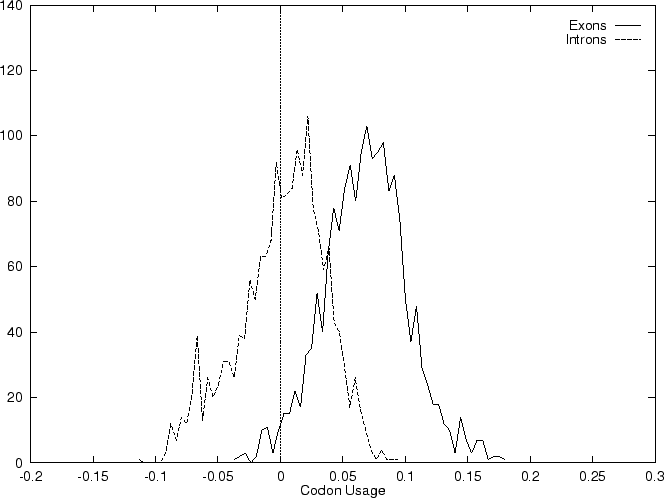
The distribution of the scores of the Codon Usage log-likelihood ratios in the larger sets of intron and exon sequences are shown below

As it is possible to see, although the distributions are clearly distinct, there is substantial overlap between the Codon Usage scores in the sets of intron and exon sequences. As we will see, this is a general situation for all coding statistics.

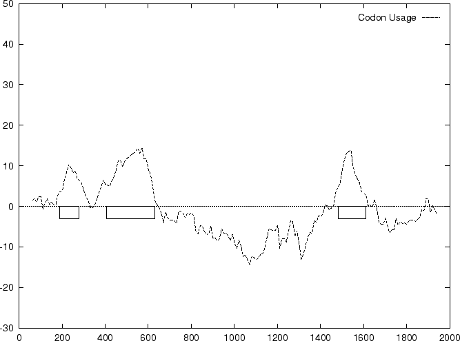
In the practice, the problem is not usually to determine the likelihood that a given sequence is coding or not, but to locate the (usually small) coding regions within large genomic sequences. The typical procedure is to compute the value of a coding statistic in successive (usually overlapping) windows (an sliding window), and record the value of the statistic for each of the windows. This generates a profile along the sequence in which peaks may point to the coding regions and valleys to the non-coding ones.

Below, we plot the result of sliding a window of length 120 bp, the distance between consecutive windows being 10 bp, computing $LP$ in the three different frames, and plotting the highest value obtained. The test sequence used is 2000 bp genomic region coding for the human $\beta$-globin gene. In this case, the codon usage log-likelihood profile reproduces fairly well the exonic structure of this gene

More information

Search by Content. Adapted from Guigo, R. ``DNA Composition, Codon Usage and Exon Prediction'' in Bishop M. ed , GENETIC DATABASES, Academic Press, 1999.